Backward Propagation Tutorial

Backward Propagation Tutorial

Introduction

Backward Propagation is probably the most common method for training forward-feed neural networks. A forward pass using an input pattern propagates through the network and produces an actual output. The backward pass uses the desired outputs corresponding to the input pattern and updates the weights according to the error signal.

There are hundreds of papers covering the subject of backward propagation. Unfortunately, many of them tend to exhibit a vast stockpile of equations and complicated partial derivatives with undefined variables to explain a concept that is really quite simple. Quite often, a pseudocode algorithm or an example with pictures is the most effiecient method to convey information.

Artificial Neuron Anatomy

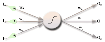
w --> weight
I --> input
O --> output
A --> activation value

Think of the activations as a pulses of electricity traveling along the dendrite path. Each activation pulse is multiplied by the weight of the dendrite it is traveling along. When all inputs to the neuron have been "stimulated" with this pulse, the neuron adds up these products and performs a thresholding or "squashing" operation on the resulting sum. The result of the squashing function is then sent to each of its output dendrites and the process is repeated for each neuron on the receiving end.

Thus, the net input of each neuron is:

(EQU 1)

Read this equation as: The net input of a neuron is the sum of (all weights connected as inputs to the neuron * all activation values of the neurons at the end of those inputs)

i refers to a neuron that is an input to the neuron we're looking at. (PREVIOUS)
j is the node we're currently looking at. (CURRENT)
k refers to a neuron that is an output to the neuron we're looking at. (NEXT)

In the above diagram, the netin for the neuron would be:

netin = (w0 * A0) + (w1 * A1) + (w2 * A2);

The Activation Function

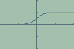
The most common squashing function is the sigmoidal function defined as:

(EQU 2) which might look something like this if you graphed it on your TI-82 using F = 5:

F is a factor that determines the pitch or "steepness" of the function's graph. The sigmoid function will take an input and "squash" it so that it's output is between 0 and 1.

So now we know how find netin for the neuron and use it to give us an activation pulse A using Act(netin).

The Forward Pass

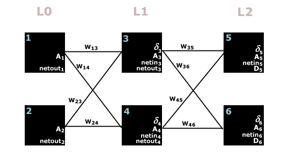
Consider the following network:

For the forward pass, the only neuron variables we are interested in are netin and A. Throughout the forward pass, all weights (W) remain constant -- the only values that ever change are netin and our activation pulse A.

Nodes 1 and 2 are input nodes.
Nodes 3 and 4 are hidden nodes.
Nodes 5 and 6 are output nodes.

The object of a forward pass is to give input nodes 1 and 2 your input pattern, and then compute netin and activation A for each node. At the end of the pass, output nodes 5 and 6 will hold activation values that essentially tell you what the network thinks the answer is.

At the start of a forward pass, nodes 1 and 2 are given input values.

Node1.A = some input pattern bit
Node2.A = some input pattern bit

Then recalling equations 1 and 2, we can compute Node3.netin and Node4.netin by the following:

(EQU 1)

Node3.netin = (Node1.A* W13) + (Node2.A * W23)
Node4.netin = (Node1.A* W14) + (Node2.A * W24)

Now that we know the netin values for neurons 3 and 4, we can use the threshold function to find their activation values.

(EQU 2)

Node3.A = 1 / (1 + e^(-F * Node3.netin))
Node4.A = 1 / (1 + e^(-F * Node4.netin))

Now we can do the exact same things we just did above to give us the activation values of neurons 5 and 6.

Node5.netin = (Node3.A * W35) + (Node4.A* W45)
Node6.netin= (Node3.A * W36) + (Node4.A* W46)

Node5.A= 1 / (1 + e^(-F * Node5.netin))
Node6.A = 1 / (1 + e^(-F * Node6.netin))

Done! A5 and A6 are the outputs of our network after a forward pass.

The Backward Pass

In the backward pass, we are given the desired outputs and propagate backward through the network updating weight values for each dendrite. You should perform a forward pass before running a backward pass. During a backward pass, the variables A and netin remain constant and the values that change are §, netout, D and W. A backward pass takes one parameter -- the desired output (D) that you think the previous input given in the forward pass should have produced as an output.

§ Is the error signal at each neuron. It emulates a pulse much like the activation value A in forward propagation.
(I couldn't find a greek delta in html -- so pretend it's the same delta in the network diagram above.)
netout is the sum of all output products for a neuron. It is much like the netin in forward propagation.
Wjk is the weight of a particular dendrite between neuron j and a neuron k that is an ouput of neuron j.
D is the given desired value (used only on ouput nodes). (as the "trainer", you provide this value)
A is the activation value that was calculated for each node during the forward pass.
netin is the sum of all input units that was calculated for each neuron during the forward pass.
F is a constant that specifies the slope/pitch of the sigmoidal function.
n (neta) is a constant that determines the learning rate of the network.

For the output nodes, netout is not computed, (there are no outputs on an output node). So for an output node, we set our netout to be the difference between our desired output and the actual output that the network gave when we did our last forward pass.

(EQU 3)

Calculating netout in our example network above for nodes 5 and 6 is as easy as:

Node5.netout = (Node5.D - Node5.A)
Node6.netout = (Node6.D - Node6.A)

To find the error signal for any neuron, we calculate an error using:

(EQU 4)

As you recall from our forward pass our sigmoidal activation function is:

(EQU 2)

Taking the derivative of Act(netin) gives us:

(EQU 5)

Substituting this into EQU 4 we get:

(EQU 4)

This simplified version is the official equation we'll use for updating our error signals (§). So, in the case of our network above, we can find the error signals of the two output nodes 5 and 6 by:

Node5.§ = Node5.A * (1 - Node5.A) * Node5.netout
Node6.§ = Node6.A * (1 - Node6.A) * Node6.netout

The error in a neuron is used to update all of its input dendrites' weights using the following equation:

(EQU 5)

Since we have the error signals Node5.§ and Node6.§ we can use this equation with neurons 3 and 4 in the diagram to update their input weights.

W35 = W35 + n * Node5.§ * Node3.A
W36 = W36 + n * Node6.§ * Node3.A
W45 = W45 + n * Node5.§ * Node4.A
W46 = W46 + n * Node6.§ * Node4.A

The method for calculating the general netout for all non-ouput nodes is much like finding the general netin on a forward pass

(EQU 6)

Implementing this with our example network diagram above, we calculate our netout variables via:

Node3.netout = (W35 * Node5.§) + (W36 * Node6.§)
Node4.netout = (W45 * Node5.§) + (W46 * Node6.§)

And use the netout variables to calculate our error signals §.

Node3.§ = Node3.A * (1 - Node3.A) * Node3.netout
Node4.§ = Node4.A * (1 - Node4.A) * Node4.netout

At this point, all equations have been introduced, and we continue back-propagating by calculating each neuron's netout and §, and then then updating its output weights until the entire network is updated. Continuing our example, we move on to nodes 1 and 2 and update their output weights as follows:

W13 = W13 + n * Node3.§ * Node1.A
W14 = W14 + n * Node4.§ * Node1.A
W23 = W23 + n * Node3.§ * Node2.A
W24 = W24 + n * Node4.§ * Node2.A

If neurons 1 and 2 were hidden nodes, we would compute their error signals, and keep going. However, since1 and 2 are input nodes and we have already updated all weights in the network, there is no need to continue. That's all there is to it!

Network Structure and Variations

Bi-connection: Most networks are bi-connected so that each layer is fully connected with the layers immediately before and after it.

Biases: To help "normalize" a neural network, most networks have bias nodes connected as an input to each non-input neuron. You initialize their dendrite weights in the same way as any other neuron, and give them an initial activation value of -1 or 1. Treat them as you would treat a neuron in the input layer and update their dendrite weights during back-propagation just as you would update the weights of any other dendrite.

Initialization: The simplest way to initialize a network's weights is using small random values, say between +- 0.5. It doesn't matter how you initialize the activation values, error signals, or any other parameters specific to a neuron because they are over-written during the propagation processes. Two guys named Nguyen and Widrow came up with an initialization scheme that seems to help the network converge a bit faster.

F = ((0.7h^(1/i))/R)
BiasWeights = +-F
All Other Weights = F

F = the weight scale factor.
R is the range of input values
h = # of hidden neurons
i = # of input neurons
w = weight

The Squashing Function: Although the most popular thresholding technique uses the sigmoidal method, there are several other functions that might yield a better result in a particular situation. Some networks such as ANFIS use a fuzzy logic lookup table to appropriately modify the type of sigmoidal function as the network is trained. As far as I know, almost all activation functions are continuous and differentiable to allow the backward propagation to calculate the gradient error signal.

Here is a variation that allows you to adjust the asymptotes of the sigmoid function so that it produces an output in any given desired range:

[(-L - H) / (1 + e^(-F * netin))] + L

L --> the low boundary
H --> the high boundary
F --> the steepness/pitch factor

Classification encoding schemes

A common use of neural networks is for classification of items. The object is to take the data from a number of known samples, enter it as inputs to the network and use backward propagation to train the network so that it later it can correctly classify each sample. So once you have the back-prop algorithms coded up, the next step is to figure out how to encode your information so that the network outputs a meaningful value. There are many ways in which you can encode your information, but there are two schemes that seem to be the most popular for class separation.

Variables

Cc is the number of classes that you want to distinguish. (Class Count)
Ci is the class index.
A is the output activation value. In this section it will always refer to the activation value of the output neuron. (METHOD 1)
{A} is a set of activation values for all output neurons (METHOD 2)
D is the given desired value for the output node (as the "trainer", you provide this value when training).

We will use an common example throughout this section. Lets say that we want the network to classify each sample as either type 0, 1, 2, 3, or 4. (5 total classes)

METHOD 1 -- One output neuron for all classes

The object here is to train the network so that the neuron's output activation value A, (usually between 0 and 1), can be divided into a specified number of classes.

=====Identification====

To get the class index Ci of a given activation value A, you would use the formula:

(EQU 7) Ci = floor(A / (1.0 / Cc))

Using our example, the following mapping shows how to convert an activation value A into the corresponding class index Ci:

A Range Class Index (Ci)
0.00-0.20 --> 0
0.21-0.40 --> 1
0.41-0.60 --> 2
0.61-0.80 --> 3
0.81-1.00 --> 4

You can use this code to convert the output neuron's activation value A into a class index Ci.

// given the output neuron's activation output (dAct), and the # of classes, return it's corresponding index
static int ClassGetIndex(double dAct, int nNumClasses) {
return (int)(dAct / (1.0 / (double)nNumClasses));
}

So for example, if the network's output node's activation value A is 0.34, then to find the corresponding index we use (EQU 7):

In our example there are 5 total classes (0 to 4), so Cc is 5.
Ci = floor(0.43 / (1.0 / 5))
Ci = 1

**note that we can easily check using the above map to see that 0.21 < 0.34 < 0.40

int nClassIdx = GetClassIndex(0.43, 5); // puts type 1 into nClassIdx.

=====Training====

When training the network, you would use the value that is in the "middle" of a class division to determine the desired value (D). When training, you know Ci, and want to find out what value D should be to ensure optimal training so that accurate identification is possible when the same inputs are used later. To get D, you would use the formula:

(EQU 8) D = (Ci * (1.0 / Cc)) + (1.0 / Cc / 2.0)

Here is a mapping table for our example:

Ci D
0 --> 0.1
1 --> 0.3
2 --> 0.5
3 --> 0.7
4 --> 0.9

You can use the following code to convert class index Ci to a desired value D

// given a class index and the # of classes, returns the "desired" value
static double ClassGetDesired(int nClassIdx, int nClassCnt) {
return (nClassIdx * (1.0 / (double)nClassCnt)) + (1.0 / (double)nClassCnt / 2.0);
}

So in our example, if you were training and you happen to know that a certain set of inputs are supposed to correspond to class index 3, you would use EQU 8 to find out what value should be used for D during backward propagation training.

In our example there are 5 total classes (0 to 4), so Cc is 5.
D = (3 * (1.0 / 5)) + (1.0 / 5 / 2.0)
D = 0.7

double dDesired = ClassGetDesired(3, 5); // puts 0.7 into dDesired

METHOD 2 -- One output neuron for each class

The object is to use multiple output neurons, where each output neuron corresponds to a specific class and the "winner" is the one with the largest value.

=====Identification====

In our example, for identification, we would use the following mapping scheme:

LLLLH --> 0
LLLHL --> 1
LLHLL --> 2
LHLLL --> 3
HLLLL --> 4

Where H is the largest value, and the L's are low values.

To get the class index Ci of a given set of activation values A, you would look at the activation value for each neuron and determine the index of the largest one. The output neuron with the highest activation value is considered the "winner".

For coding, lets put each output neuron's activation value into a slot in a dynamically allocated array. Then we can find the largest value in the array and get its index to convert an activation value A into a class index Ci.

// given the neural network's outputs, and # of classes,
// returns the class index that most closely matches the neural nets outputs
//
// ex: given [0.001][0.0012][0.987][0.0211], nClassCnt == 4, returns 2 since the value of index 2 is the largest
static int ClassGetIndex(double* Outputs, int nClassCnt) {
          double dLargestVal =DBL_MIN;
          int nLargestIdx = 0;
          for (int I = 0; I < nClassCnt; I++) {
                    if (Outputs[I] > dLargestVal) { dLargestVal = Outputs[I]; nLargestIdx = I; }
          }
          return nLargestIdx;
}

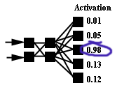
So for example if the 5 output neuron activation values {A} are:

0 1 2 3 4
{0.01, 0.05, 0.98, 0.13, 0.02}

The corresponding class index Ci would be 2 since 0.98 is the largest value and is in slot 2.

=====Training====

For training, you would simply give a desired value D of 1 for the neuron corresponding to the index you want to activate with the given training pattern, and 0 for all the other neurons.

0 --> 00001
1 --> 00010
2 --> 00100
3 --> 01000
4 --> 10000

Say you want the network to output class index Ci of type 3 for a given input set. The output nodes should use the desired values of {0, 0, 0, 1, 0} for
back-propagation.

I use the following C++ functions to translate between desired and activation values when using METHOD 2:
**Note, strings are used instead of arrays here because most of the time they're in string format being read from/written to a file. The strings could easily be replaced with an array or a list.

// given a class index and the # of classes,
// returns a string containing the desired outputs separated by strDelim
// (this is usually written to a training file)
// ex: given nClassIdx == 2, nClassCnt = 4, strDelim = "¦" --> returns "0¦0¦1¦0"
static CString ClassGetOutputString(int nClassIdx, int nClassCnt, CString strDelim) {
          CString strRet = "";
          for (int I = 0; I < nClassCnt - 1; I++) {
                    if (nClassIdx == I) { strRet += "1" + strDelim; } else { strRet += "0" + strDelim; }
          }
          if (nClassIdx == I) { strRet += "1"; } else { strRet += "0"; }
          return strRet;
}

// given a string such as "0¦0¦1¦0", returns 2 because the 1 corresponds to index 2
// returns -1 on error
static int ClassGetOutputIndex(CString strOutputs) {
          int nNum = 0; char ch;
          for (int I = 0; I < strOutputs.GetLength(); I++) {
                    ch = strOutputs[I];
                    if (ch == '1') { return nNum; } else if (ch == '0') { nNum++; }
          }
          return -1;
}

Conclusion

I've found that METHOD 2 seems to be more accurate for most applications, but it requires more nodes, which increases memory requirements. METHOD 2 is also less susceptible to precision round-off error. As for speed, I'm not sure which one trains faster. Each epoch takes longer using METHOD 2, but METHOD 2 doesn't seem to require as many epochs to get a good separation.

Additional Introductory Information

http://home.cc.umanitoba.ca/~umcorbe9/perceptron.html A perceptron java applet that lets you step through an example.
http://www.dontveter.com/bpr/public2.html -- walks through an example of the XOR network. I found it extremely helpful. Sometimes an example is worth more than 1000 greek variables.
http://www.ece.ubc.ca/~elec592/PDFfiles/7.0.pdf -- gives some insight as to how the back-propagation method is derived, although I think it's a bit of an overkill.

Questions, comments, or fixes can be sent to lclemens@gmail.com

Luke Clemens
February 15, 2002
http://clemens.bytehammer.com